hands-on exercise 2

Beyond ggplot2 Fundamentals

pacman::p_load(ggrepel, patchwork, 
               ggthemes, hrbrthemes,
               tidyverse )

exam_data <- read_csv("data/Exam_data.csv")

the plot

code chunk

ggplot(data=exam_data, 
       aes(x= MATHS, 
           y=ENGLISH)) +
  geom_point() +
  geom_smooth(method=lm, 
              size=0.5) +  
  geom_label(aes(label = ID), 
             hjust = .5, 
             vjust = -.5) +
  coord_cartesian(xlim=c(0,100),
                  ylim=c(0,100)) +
  ggtitle("English scores versus Maths scores for Primary 3")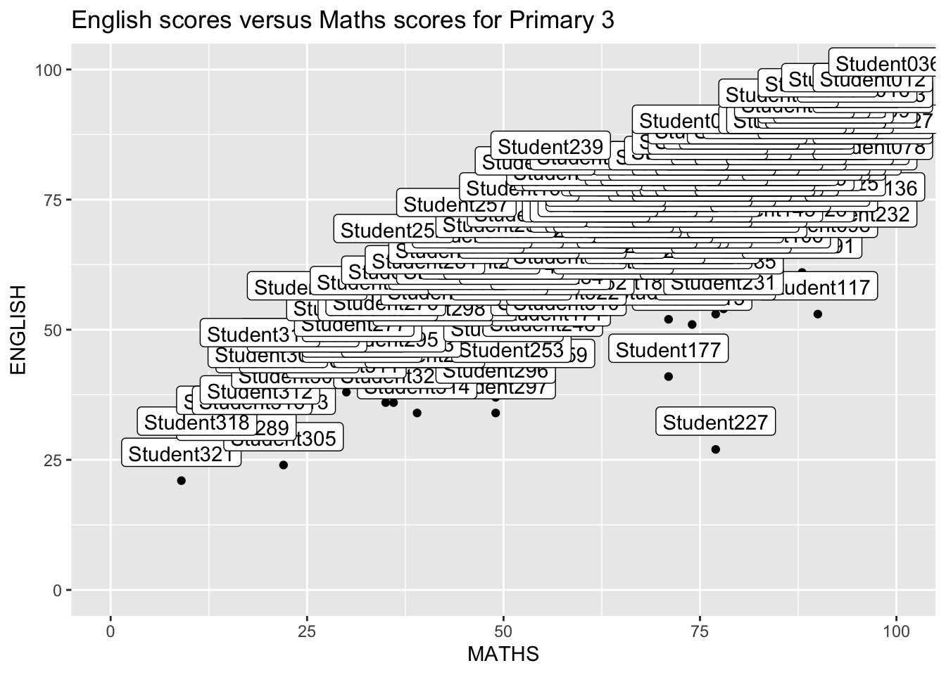

ggplot(data=exam_data, 
       aes(x= MATHS, 
           y=ENGLISH)) +
  geom_point() +
  geom_smooth(method=lm, 
              size=0.5) +  
  geom_label_repel(aes(label = ID), 
                   fontface = "bold") +
  coord_cartesian(xlim=c(0,100),
                  ylim=c(0,100)) +
  ggtitle("English scores versus Maths scores for Primary 3")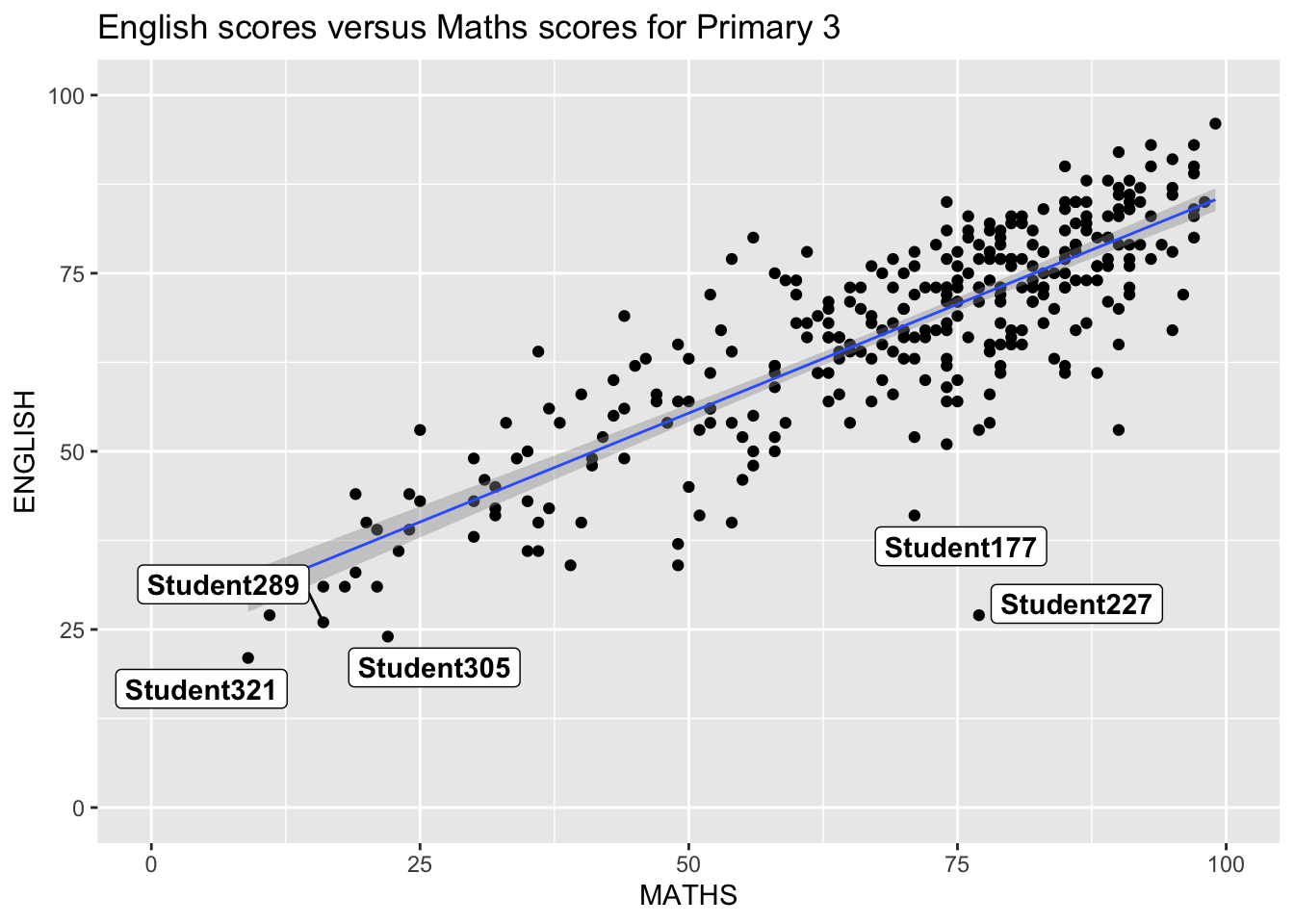

Expalintation: “ggrepel” is designed to address the issue of overlapping between labels in charts and graphics. It automatically adjusts the positions of text labels to prevent overlap, thereby enhancing the clarity and readability of the graphics.

ggplot(data=exam_data, 
             aes(x = MATHS)) +
  geom_histogram(bins=20, 
                 boundary = 100,
                 color="grey25", 
                 fill="grey90") +
  theme_gray() +
  ggtitle("Distribution of Maths scores")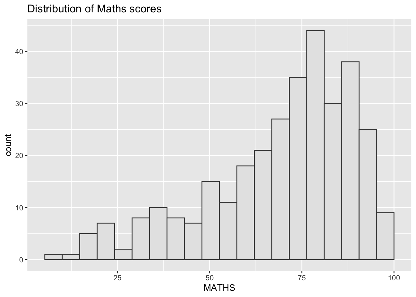 

ggplot(data=exam_data, 
             aes(x = MATHS)) +
  geom_histogram(bins=20, 
                 boundary = 100,
                 color="grey25", 
                 fill="grey90") +
  ggtitle("Distribution of Maths scores") +
  theme_economist()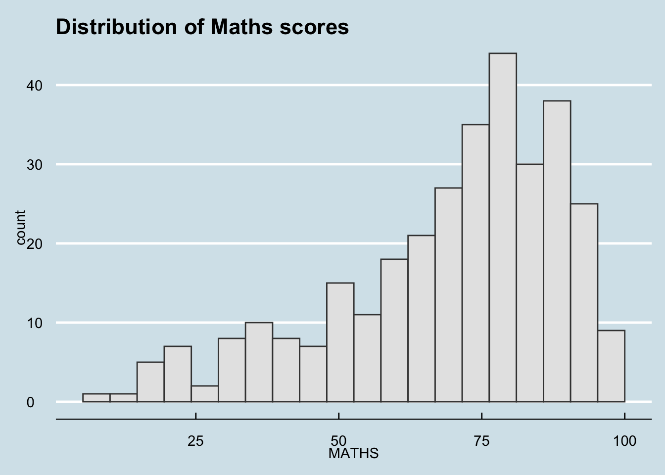

Explaination:“Themes” are about styling and mainly help in enhancing the overall appearance of charts, making them more readable and aesthetically pleasing.

ggplot(data=exam_data, 
             aes(x = MATHS)) +
  geom_histogram(bins=20, 
                 boundary = 100,
                 color="grey25", 
                 fill="grey90") +
  ggtitle("Distribution of Maths scores") +
  theme_ipsum()

ggplot(data=exam_data, 
             aes(x = MATHS)) +
  geom_histogram(bins=20, 
                 boundary = 100,
                 color="grey25", 
                 fill="grey90") +
  ggtitle("Distribution of Maths scores") +
  theme_ipsum(axis_title_size = 18,
              base_size = 15,
              grid = "Y")

Explaination: The ‘hrbrthemes’ package in R primarily provides additional themes and styles, offering tools for customization and beautification

p1 <- ggplot(data=exam_data, 
             aes(x = MATHS)) +
  geom_histogram(bins=20, 
                 boundary = 100,
                 color="grey25", 
                 fill="grey90") + 
  coord_cartesian(xlim=c(0,100)) +
  ggtitle("Distribution of Maths scores")

p2 <- ggplot(data=exam_data, 
             aes(x = ENGLISH)) +
  geom_histogram(bins=20, 
                 boundary = 100,
                 color="grey25", 
                 fill="grey90") +
  coord_cartesian(xlim=c(0,100)) +
  ggtitle("Distribution of English scores")

ggplot(data=exam_data, 
             aes(x = MATHS)) +
  geom_histogram(bins=20, 
                 boundary = 100,
                 color="grey25", 
                 fill="grey90") +
  ggtitle("Distribution of Maths scores") +
  theme_economist()

ggplot(data=exam_data, 
             aes(x = MATHS)) +
  geom_histogram(bins=20, 
                 boundary = 100,
                 color="grey25", 
                 fill="grey90") +
  ggtitle("Distribution of Maths scores") +
  theme_ipsum()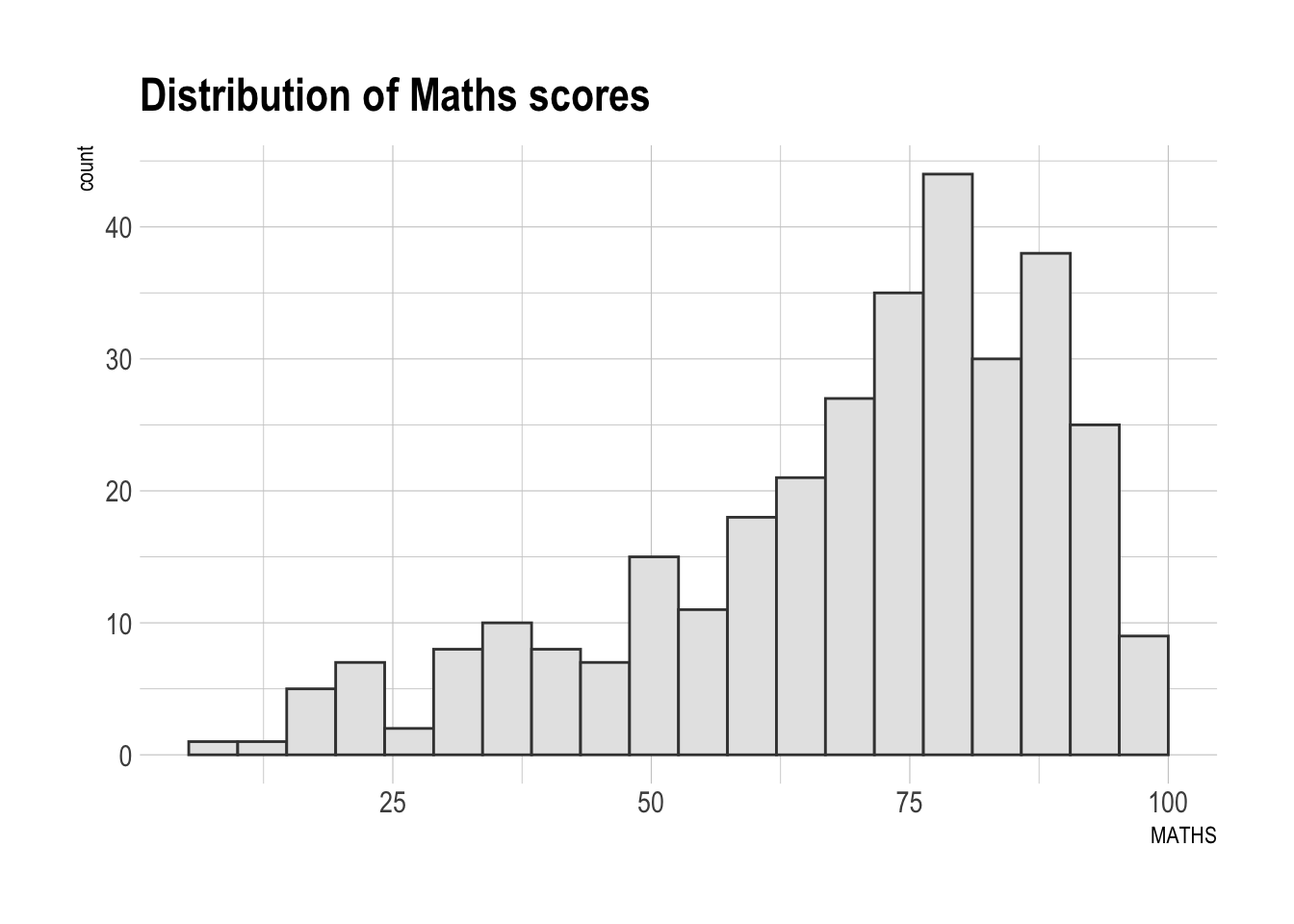

ggplot(data=exam_data, 
             aes(x = MATHS)) +
  geom_histogram(bins=20, 
                 boundary = 100,
                 color="grey25", 
                 fill="grey90") +
  ggtitle("Distribution of Maths scores") +
  theme_ipsum(axis_title_size = 18,
              base_size = 15,
              grid = "Y")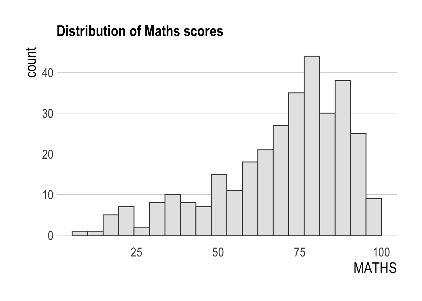

Explaination: In R, a ‘Single Graph’ primarily refers to an independent chart, mainly used for displaying specific data or handling data relationships.

p1 <- ggplot(data=exam_data, 
             aes(x = MATHS)) +
  geom_histogram(bins=20, 
                 boundary = 100,
                 color="grey25", 
                 fill="grey90") + 
  coord_cartesian(xlim=c(0,100)) +
  ggtitle("Distribution of Maths scores")

p2 <- ggplot(data=exam_data, 
             aes(x = ENGLISH)) +
  geom_histogram(bins=20, 
                 boundary = 100,
                 color="grey25", 
                 fill="grey90") +
  coord_cartesian(xlim=c(0,100)) +
  ggtitle("Distribution of English scores")

p3 <- ggplot(data=exam_data, 
             aes(x= MATHS, 
                 y=ENGLISH)) +
  geom_point() +
  geom_smooth(method=lm, 
              size=0.5) +  
  coord_cartesian(xlim=c(0,100),
                  ylim=c(0,100)) +
  ggtitle("English scores versus Maths scores for Primary 3")

p1 + p2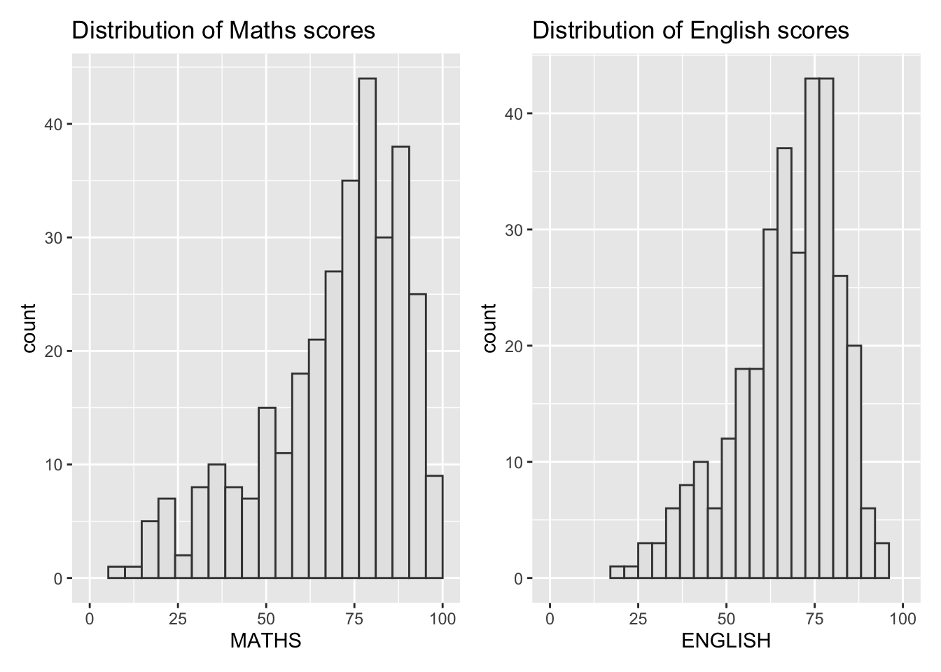

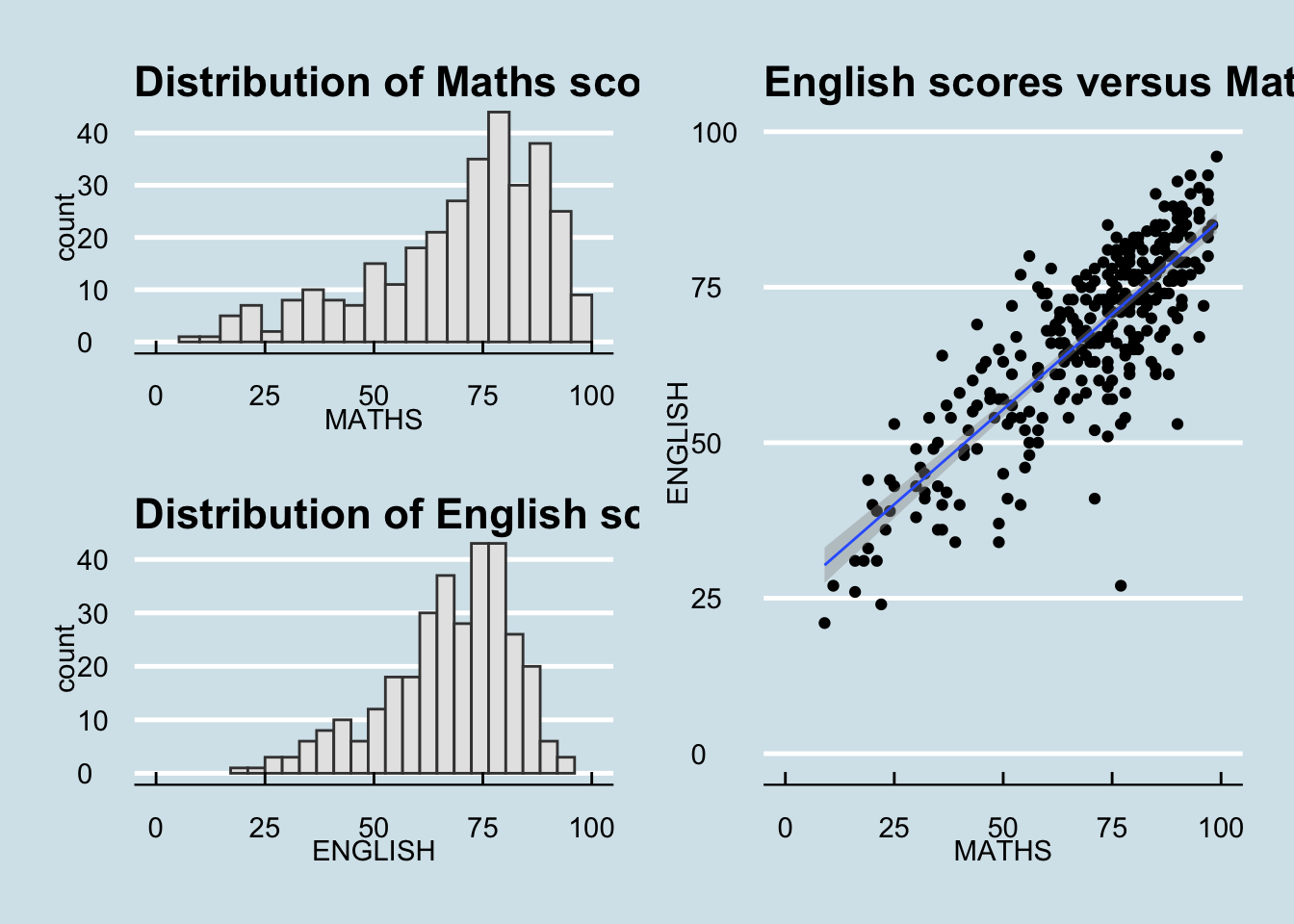
(p1 / p2) | p3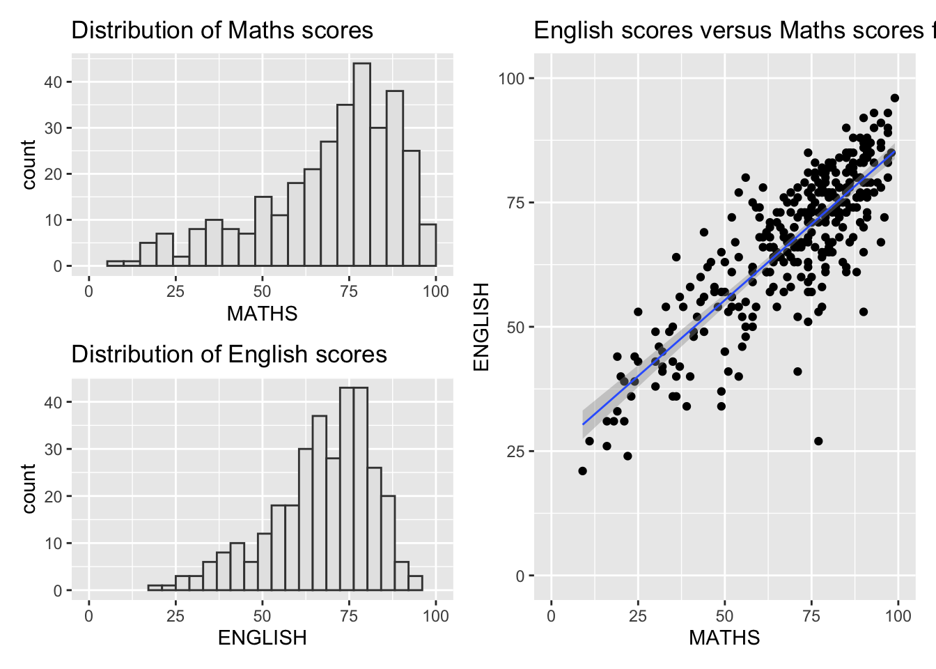

((p1 / p2) | p3) + 
  plot_annotation(tag_levels = 'I')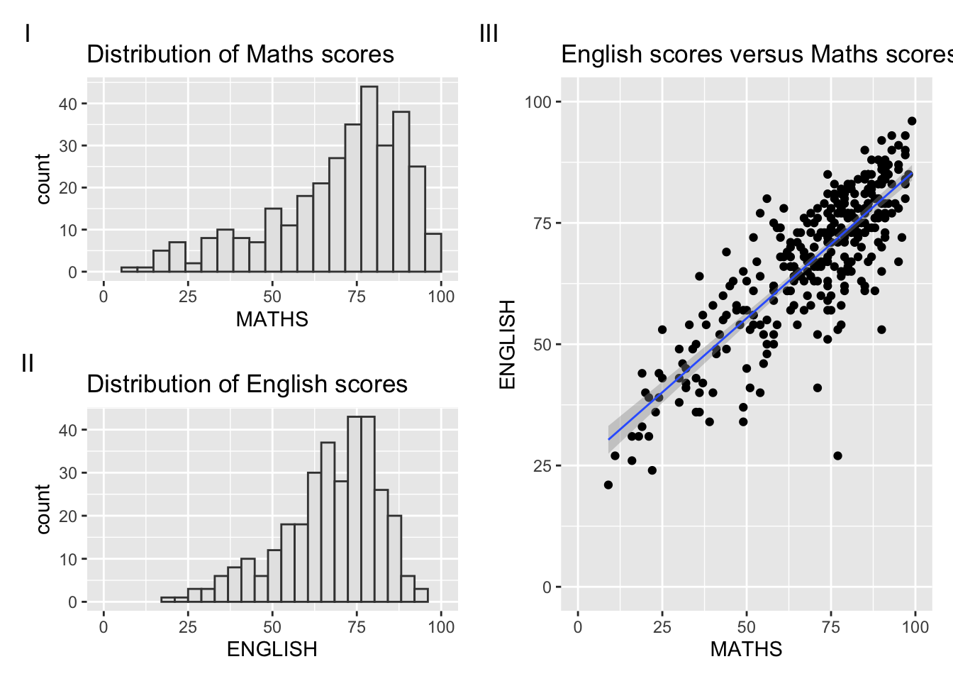

p3 + inset_element(p2, 
                   left = 0.02, 
                   bottom = 0.7, 
                   right = 0.5, 
                   top = 1)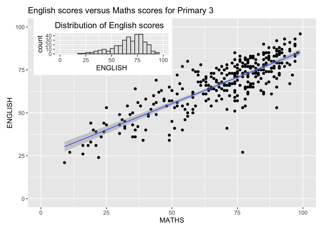

patchwork <- (p1 / p2) | p3
patchwork & theme_economist()

Expalination: In R, ‘patchwork methods’ combine multiple charts, offer flexible layout control, simplify the process of chart combination, and allow for high customization.